1️⃣ 背景与目标

B样条轨迹因其光滑、连续、可微等特性，广泛应用于无人系统路径规划中。然而，若控制点分布不合理，曲线可能出现剧烈弯折（高曲率），影响可控性与执行安全性。

我们将引入一个 “二阶差分曲率代价项”，控制曲线局部变化，优化过程自动平滑高曲率段，提升轨迹质量。

2️⃣ 二阶差分与曲率

在离散控制点层面，曲率近似由二阶差分向量表达：

💡 二阶差分定义：

• 表示相邻三个控制点的“折线弯曲程度”
• 二阶差分越大，说明控制点形成更尖锐的弯折，对应曲线曲率大

⚠️ 注意事项：

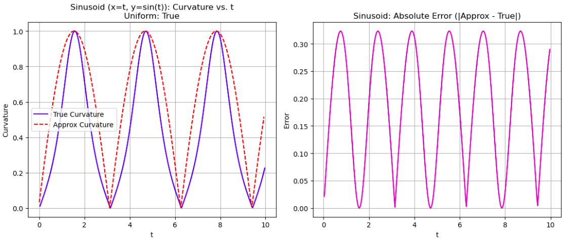
该二阶差分项并不是真正的几何曲率(实际上是加速度)，而是一种简化的近似。在以下假设成立时，它才能较好地反映曲率趋势：

• 控制点之间 间距较小且均匀
• B 样条参数 t 与弧长 近似线性关系
• 曲线采样点分布 近似等距

但是依然有一定的误差，如下图所示：

3️⃣ 曲率代价函数设计

设定最大允许曲率（差分范数）为 ​\kappa_{\text{max}}，一旦超限，则施加惩罚代价。

📦 代价项定义：

对于每组三个控制点：

最终总曲率代价为：

4️⃣ 可导性与梯度推导

✅ 由于我们使用的是范数 + 二次惩罚项，整体函数连续可导，适用于主流优化器。

✏️ 梯度推导（链式法则）：

对 ​\mathbf{d}_2 = \mathbf{P}_i - 2\mathbf{P}_{i+1} + \mathbf{P}_{i+2}：

再对控制点求偏导（线性关系）：

其中：

5️⃣ C++ 实现代码

// 计算曲率成本及其梯度（二维）
// 若某个二阶差分超出阈值，则添加代价，并更新梯度
void BsplineOptimizer::calcCurvatureCost(
    const Eigen::MatrixXd& ctrl_points,
    double& cost,
    std::vector<double>& grad) 
{
    cost = 0.0;
    int num_ctrl_points = ctrl_points.cols();

    for (int i = 0; i < num_ctrl_points - 2; ++i) {
        Eigen::Vector2d d2 = ctrl_points.col(i) 
                           - 2 * ctrl_points.col(i + 1) 
                           + ctrl_points.col(i + 2);
        double norm_d2 = d2.norm();

        if (norm_d2 > max_curvature_) {
            double penalty = norm_d2 - max_curvature_;
            cost += penalty * penalty;

            Eigen::Vector2d grad_term = (2.0 * penalty / norm_d2) * d2;

            grad[2 * i + 0]     += grad_term.x();
            grad[2 * i + 1]     += grad_term.y();
            grad[2 * (i + 1) + 0] += -2.0 * grad_term.x();
            grad[2 * (i + 1) + 1] += -2.0 * grad_term.y();
            grad[2 * (i + 2) + 0] += grad_term.x();
            grad[2 * (i + 2) + 1] += grad_term.y();
        }
    }
}

6️⃣ Python 动画可视化

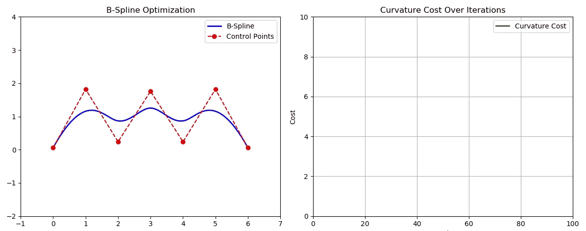
import numpy as np
import matplotlib.pyplot as plt
from matplotlib.animation import FuncAnimation
from scipy.interpolate import BSpline

# 控制参数
max_curvature = 1.0
num_iters = 100
alpha = 0.01  # 梯度步长

# 初始化控制点
ctrl_pts = np.array([
    [0, 0],
    [1, 2],
    [2, 0],
    [3, 2],
    [4, 0],
    [5, 2],
    [6, 0]
], dtype=float)

# B样条阶数（这里取3阶）
k = 3
n = len(ctrl_pts)
t = np.concatenate((
    np.zeros(k),
    np.linspace(0, 1, n - k + 1),
    np.ones(k)
))

# 计算B样条点
def get_bspline(ctrl_pts):
    spline = BSpline(t, ctrl_pts, k)
    x = np.linspace(0, 1, 200)
    pts = spline(x)
    return pts[:, 0], pts[:, 1]

# 计算二阶差分曲率代价和梯度
def curvature_cost_and_grad(ctrl_pts, max_curvature):
    cost = 0.0
    grad = np.zeros_like(ctrl_pts)
    for i in range(len(ctrl_pts) - 2):
        d2 = ctrl_pts[i] - 2 * ctrl_pts[i+1] + ctrl_pts[i+2]
        norm_d2 = np.linalg.norm(d2)
        if norm_d2 > max_curvature:
            penalty = norm_d2 - max_curvature
            cost += penalty ** 2
            grad_term = (2.0 * penalty / norm_d2) * d2
            grad[i]     += grad_term
            grad[i+1]   += -2.0 * grad_term
            grad[i+2]   += grad_term
    return cost, grad

# 初始化画布：左图B样条 + 右图代价图
fig, (ax_curve, ax_cost) = plt.subplots(1, 2, figsize=(12, 5))

spline_line, = ax_curve.plot([], [], 'b-', lw=2, label='B-Spline')
ctrl_line, = ax_curve.plot([], [], 'ro--', label='Control Points')
ax_curve.set_xlim(-1, 7)
ax_curve.set_ylim(-2, 4)
ax_curve.set_title("B-Spline Optimization")
ax_curve.legend()

# cost 曲线初始化
cost_values = []
cost_line, = ax_cost.plot([], [], 'g-', label='Curvature Cost')
ax_cost.set_xlim(0, num_iters)
ax_cost.set_ylim(0, 10)  # 初始范围，动态调整可加
ax_cost.set_title("Curvature Cost Over Iterations")
ax_cost.set_xlabel("Iteration")
ax_cost.set_ylabel("Cost")
ax_cost.grid(True)
ax_cost.legend()

def init():
    return spline_line, ctrl_line, cost_line

def animate(i):
    global ctrl_pts, cost_values
    cost, grad = curvature_cost_and_grad(ctrl_pts, max_curvature)
    ctrl_pts -= alpha * grad  # 梯度下降

    x_spline, y_spline = get_bspline(ctrl_pts)
    spline_line.set_data(x_spline, y_spline)
    ctrl_line.set_data(ctrl_pts[:, 0], ctrl_pts[:, 1])

    # 更新 cost 曲线
    cost_values.append(cost)
    cost_line.set_data(range(len(cost_values)), cost_values)
    ax_cost.set_ylim(0, max(1.0, max(cost_values)) * 1.1)

    return spline_line, ctrl_line, cost_line

ani = FuncAnimation(fig, animate, frames=num_iters, init_func=init, blit=True, interval=500)
plt.tight_layout()
plt.show()